Final Project: Prediciting Head to Head Pokémon Wins with Multi-level Binary Logistic Regression

PSY-504

Final-Project

Coding

Tutorial

Author

Affiliation

Steven Mesquiti

Princeton University

Overview

This tutorial will walk you through the process of simulating Pokémon battles using the OpenAI API and then analyzing the results using a multi-level binary logistic regression model using a Specification Curve Analysis framework. The main analytic goal is to see which Pokemon stats are most predictive of winning a battle.

We are using a multi-level binary logistic regression model given the multiple levels of data we have. Each battle is a unique observation, but each Pokémon has multiple stats that are used to predict the outcome of the battle. This means that we need to account for the fact that different Pokémon may have different effects on the outcome of the battle. Further, we have to employ a logistic regression framework since our outcome is binary (win/loss).

Load packages:

if(!require('pacman')) {
    install.packages('pacman')
}
library(pacman)
pacman::p_load(tidyverse, DT, broom, performance,
               ordinal,car,ggeffects,gofact,lme4,
               emmeans,knirt,MASS,brant,devtool,purr,GGally,
               specr, furrr,install = TRUE)
devtools::install_github("hadley/emo")

#### define plot objects and stuff

palette <- c(
  "#772e25", "#c44536", "#ee9b00", "#197278", "#283d3b", 
  "#9CC5A1", "#6195C6", "#ADA7C9", "#4D4861", "grey50",
  "#d4a373", "#8a5a44", "#4a6a74", "#5c80a8", "#a9c5a0",
  "#7b9b8e", "#e1b16a", "#a69b7c", "#9d94c4", "#665c54"
)

palette_condition = c("#ee9b00", "#c44536","#005f73", "#283d3b", "#9CC5A1", "#6195C6", "#ADA7C9", "#4D4861")

plot_aes = theme_minimal() +
  theme(
    legend.position = "top",
    legend.text = element_text(size = 12),
    text = element_text(size = 16, family = "Futura Medium"),
    axis.text = element_text(color = "black"),
    axis.ticks.y = element_blank(),
    plot.title = element_text(size = 20, hjust = 0.5) # Adjusted title size and centering
  )

GPT Pipeline

First, before we conduct any statistical analyses, we will use the OpenAI API to simulate Pokémon battles. This will allow us to create a dataset of battle outcomes based on Pokémon stats. We are going to use gpt-3.5-turbo to simulate the battles. Given that this is a rather simple task, we don’t need to leverage a terribly complex or powerful model (e.g., gpt-4).

Load Libraries, API Key, and set model information

Start by loading in the necessary libraries (and installing them if necessary) and setting up the OpenAI API key. I’d recommend running this in a separate notebook, as it will take a while to run the ~3000 individual battles. We also set a temperature of 0 to make the model more deterministic.

💡 It is important to note that you should not share your OpenAI API key with anyone. It is a sensitive piece of information that should be kept private. If you are using a public notebook or sharing your code, make sure to remove or mask your API key before sharing. You can use environment variables or a .env file to store your API key securely.

from openai import OpenAI, RateLimitError, APIError, APITimeoutError
import pandas as pd 
from tqdm.notebook import tqdm
from dotenv import load_dotenv
import re
import numpy as np
import json
import argparse
import random
import time
import os
import ast

load_dotenv("/Users/sm9518/Desktop/Article-Summarizer/.env") # where i keep my API key... 
api_key = os.getenv("OPENAI_API_KEY")
if api_key:
    print("API Key loaded successfully!\n:)")
else:
    raise ValueError("API Key not found.\nMake sure it is set in the .env file.")
model="gpt-3.5-turbo" # set model. we dont need anything fancy for this task.
temperature=0 # set temp to be rather determinisitic 
SEED = random.seed(42) # set seed for reproducibility

Load Data and Sample

Before we run the simulations, we have to create our dataset. This can be done by downloading the original kaggle dataset here.

Once you’ve done so, we will extract the original 151 Pokémon and create a dataset of 20 matchups for each Pokémon.

df = pd.read_csv('/Users/sm9518/Library/CloudStorage/GoogleDrive-sm9518@princeton.edu/My Drive/Classes/Stats-blog/posts/final-project/data/pokedex.csv', index_col=0)
df.head()

OG_pokedex = df.iloc[:151].copy() # take the OG 151 pokemon

# build the 20‐matchups per Pokémon
matchups = []
for challenger in OG_pokedex['name']:
    pool = [p for p in OG_pokedex['name'] if p != challenger]
    opponents = random.sample(pool, 20) # give them 20 challengers
    for opponent in opponents:
        matchups.append({'challenger': challenger, 'opponent': opponent})
matchups_df = pd.DataFrame(matchups)



# merge challenger metadata
matchups_with_meta = (
    matchups_df
    .merge(
        OG_pokedex.add_suffix('_challenger'),
        left_on='challenger',
        right_on='name_challenger',
        how='left'
    )
    # drop the redundant name_challenger column if you like
    .drop(columns=['name_challenger'])
    # merge opponent metadata
    .merge(
        OG_pokedex.add_suffix('_opponent'),
        left_on='opponent',
        right_on='name_opponent',
        how='left'
    )
    .drop(columns=['name_opponent'])
)

# now every row has both challenger_* and opponent_* columns
matchups_with_meta.head()

Hit the API to Simulate Match-ups

Once we’ve created the dataset, we can use the OpenAI API to simulate the match-ups. In short, for each battle, we will feed the stats of both Pokémon and ask GPT to determine the winner. We can then extract and save that data for downstream analyses.

💡 The API call is rate limited, so we need to be careful about how many requests we send. We will use the tqdm library to show a progress bar and add a sleep time between requests to avoid hitting the rate limit.

Our prompt is as follows:

    "Based on the stats, which Pokémon would win a one-on-one battle?\n\n"
    f"{p1_stats}\nVS\n\n{p2_stats}\n\n"
    "Only respond with the name of the winning Pokémon."

# Initialize OpenAI client
client = OpenAI()
# ---- Utility Functions ---- #

def safe_parse_types(val):
    if isinstance(val, list):
        return val
    try:
        return ast.literal_eval(val)
    except Exception:
        return [str(val)]

def format_pokemon_stats(name, row, suffix):
    types = safe_parse_types(row[f'type{suffix}'])
    return (
        f"{name.title()}:\n"
        f"- Type: {', '.join(types)}\n"
        f"- HP: {row[f'hp{suffix}']}\n"
        f"- Attack: {row[f'attack{suffix}']}\n"
        f"- Defense: {row[f'defense{suffix}']}\n"
        f"- Special Attack: {row[f's_attack{suffix}']}\n"
        f"- Special Defense: {row[f's_defense{suffix}']}\n"
        f"- Speed: {row[f'speed{suffix}']}\n"
    )

# ---- API Interaction ---- #

def get_completion(prompt):
    messages = [{"role": "user", "content": prompt}]
    response = client.chat.completions.create(
        model=model,
        messages=messages,
        temperature=temperature
    )
    return response.choices[0].message.content.strip()

def get_response(prompt):
    try:
        return get_completion(prompt)
    except RateLimitError as e:
        retry_time = getattr(e, 'retry_after', 30)
        print(f"Rate limit exceeded. Retrying in {retry_time} seconds...")
        time.sleep(retry_time)
        return get_response(prompt)
    except APIError as e:
        print(f"API error occurred: {e}. Retrying in 30 seconds...")
        time.sleep(30)
        return get_response(prompt)
    except APITimeoutError as e:
        print(f"Request timed out: {e}. Retrying in 10 seconds...")
        time.sleep(10)
        return get_response(prompt)
    except Exception as e:
        print(f"Unexpected error: {e}. Retrying in 10 seconds...")
        time.sleep(10)
        return get_response(prompt)

# ---- Simulate One Battle ---- #

def simulate_battle(row):
    p1_stats = format_pokemon_stats(row['challenger'], row, '_challenger')
    p2_stats = format_pokemon_stats(row['opponent'], row, '_opponent')

    prompt = (
        "Based on the stats, which Pokémon would win a one-on-one battle?\n\n"
        f"{p1_stats}\nVS\n\n{p2_stats}\n\n"
        "Only respond with the name of the winning Pokémon."
    )

    response = get_response(prompt)
    return response.lower()

# ---- Run All Simulations ---- #

# This should be your DataFrame containing all matchups
# matchups_with_meta = pd.read_csv(...)  # Load your data here

results = []

for idx, row in tqdm(matchups_with_meta.iterrows(), total=len(matchups_with_meta), desc="Simulating battles"):
    print(f"Simulating battle {idx + 1} of {len(matchups_with_meta)}: {row['challenger']} vs {row['opponent']}")
    winner = simulate_battle(row)
    results.append({
        "challenger": row['challenger'],
        "opponent": row['opponent'],
        "winner": winner
    })
    time.sleep(1.5)  # Respect rate limits

# ---- Save Results ---- #

results_df = pd.DataFrame(results)
matchups_with_results = matchups_with_meta.merge(
    results_df,
    on=["challenger", "opponent"],
    how="left"
)
matchups_with_results.head()
matchups_with_results.to_csv(f"/Users/sm9518/Library/CloudStorage/GoogleDrive-sm9518@princeton.edu/My Drive/Classes/Stats-blog/posts/final-project/data/pokemon_battle_results_{model}_{SEED}_{temperature}.csv", index=False)
print(f"\nDone! Winners saved to pokemon_battle_results_{model}_{SEED}_{temperature}.csv.")

Load Curated Dataset

Now that we have our dataset, we can load it in and do some basic data cleaning. We will drop the text columns and the opponent information, as we are not interested in that. We will also scale the data to make it easier to interpret when modeling

💡 For the sake of simplicity, we are only interested in the challenger Pokemon’s stats.

path = '~/Library/CloudStorage/GoogleDrive-sm9518@princeton.edu/My Drive/Classes/Stats-blog/posts/final-project/data'
df = read_csv(file.path(path, 'pokemon_battle_results_gpt-3.5-turbo_None_0.csv')) 

df_small <- df |> 
  dplyr::select(-dplyr::matches(c("info_"))) |> #drop the text col and the opponent info, we aren't interested in that
  mutate(
    winner = ifelse(winner == challenger, 1, 0),
    winner = factor(winner, levels = c(0, 1), labels = c("Loss", "Win")),
    challenger = as.factor(challenger),
    opponent = as.factor(opponent),
  ) |> 
  rename_with(~ str_replace(., "_challenger$", ""), ends_with("_challenger")) # rename the challenger variable 

df_small_scaled <- df_small %>%
  mutate(across(c(height, weight, hp, attack, defense, s_attack, s_defense, speed,
                  height_opponent, weight_opponent, hp_opponent, attack_opponent,
                  defense_opponent, s_attack_opponent, s_defense_opponent, speed_opponent), 
                scale))

Take a look at the data

Here, we are taking a look at a random sample of the data to see if it looks like we expect. We can also use the DT package to create an interactive table that allows us to sort and filter the data.

df_small |> 
  sample_n(10) |>
  DT::datatable()

Exploratory Data Analysis

Now, we can start to explore the data. We will start by looking at the distribution of the various Pokémon stats. We will also look at the relationship between the stats and the outcome of the battle (win/loss). This will help us understand how the different stats relate to each other and to winning or losing a battle.

Visualize the distribution of the various Pokémon stats

Distribution of Pokémon stats

From looking at the density plots we have some interesting insights. For example, we can see that the distribution of the Pokémon stats is not normal, and that there are some outliers in the data. We’ll leave them in since we are interested in the relationship between the stats and the outcome of the battle and know this is how the Pokemon appear in the game.

df_small |> 
  dplyr::select(3:12,-type) |> 
  pivot_longer(cols = everything(), names_to = "stat", values_to = "value") |> 
  ggplot(aes(x = value, fill = stat)) +
  geom_density(alpha = 0.7) +
  facet_wrap(~ stat, scales = "free",ncol = 3) +
  labs(title = "Distribution of Pokémon Stats", x = "Value", y = "Density") +
  scale_fill_manual(values = palette) +
  plot_aes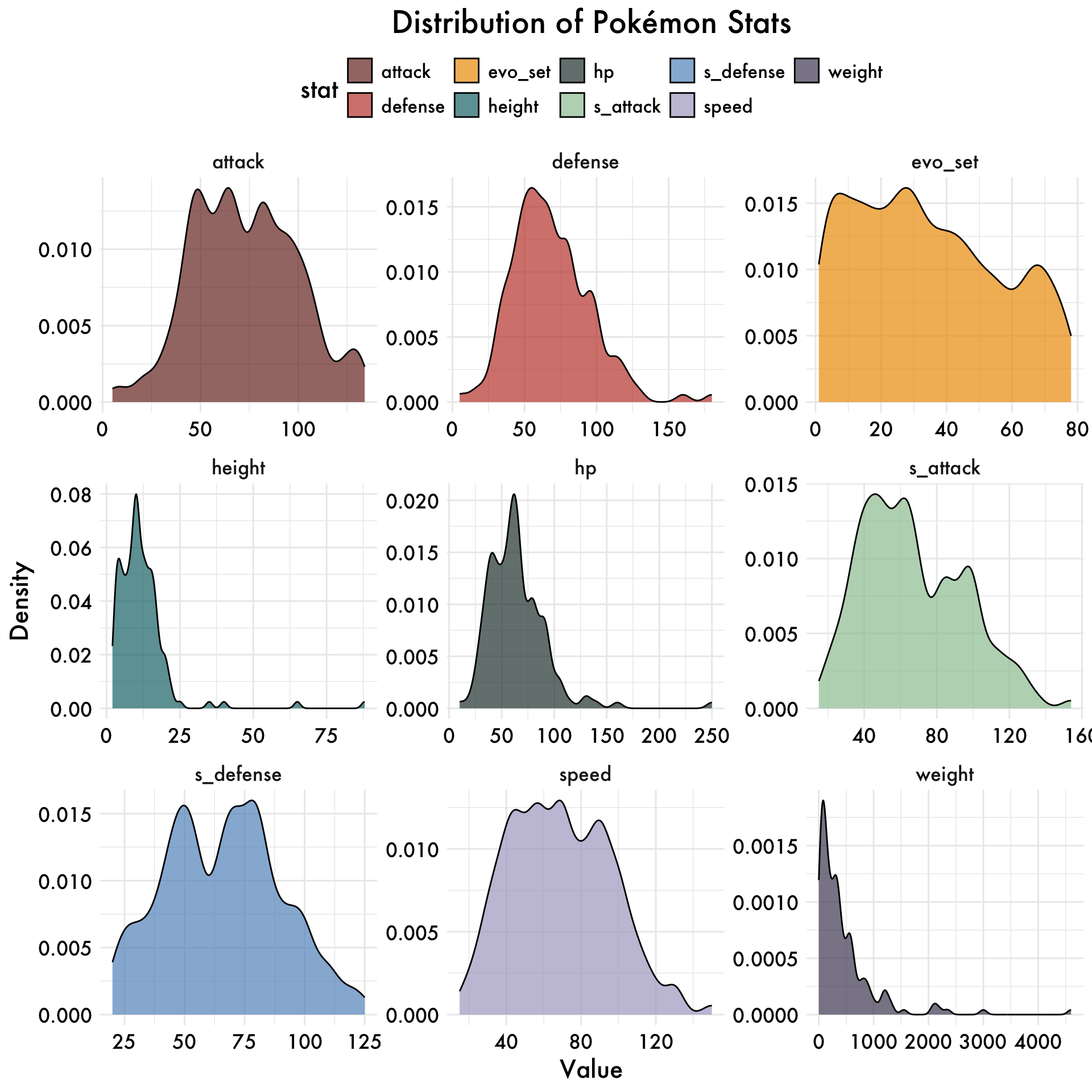

Comparing Distributions of Pokémon stats by outcome

Now, let’s look at the distribution of the Pokémon stats by winner. This will allow us to see if there are any differences in the different distributions between the winners and losers without running any analyses

df_small |> 
  dplyr::select(3:12, -type, winner) |> 
  rename(outcome = winner) |> 
  pivot_longer(cols = -outcome, names_to = "stat", values_to = "value") |> 
  ggplot(aes(x = value, fill = outcome)) +
  geom_density(alpha = 0.7) +
  facet_wrap(~ stat, scales = "free", ncol = 3) +
  labs(title = "Distribution of Pokémon Stats by Battle Outcome", 
       x = "Value", y = "Density") +
  scale_fill_manual(values = c("Win" = "#4daf4a", "Loss" = "#e41a1c")) +
  plot_aes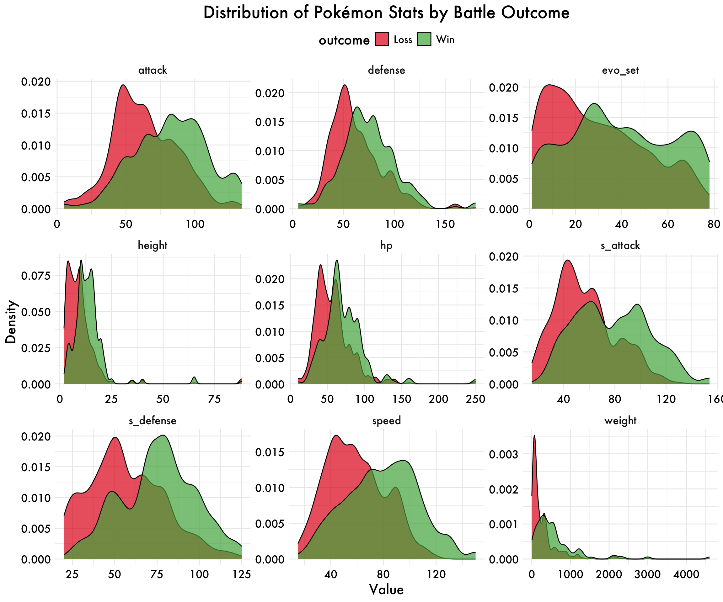

Comparing Relations between variables and outcomes

This plot shows how different Pokémon stats relate to each other and to winning or losing a battle. The diagonal panels show how each stat is distributed for winners (green) and losers (red). The lower panels show relationships between pairs of stats, with trendlines and points colored by outcome. The upper panels give the strength of the relationship between each pair of stats. Look for where the green and red separate—those are the stats or stat combinations most associated with winning or losing.

# Define your color palette
my_colors <- c("Win" = "#4daf4a", "Loss" = "#e41a1c")

df_small %>%
  dplyr::select(3:12, -type, winner) %>%
  rename(outcome = winner) |> 
  ggpairs(
    columns = 1:9,  # Excludes winner column from variables
    mapping = aes(color = outcome, alpha = 0.2),
    lower = list(
      continuous = wrap("smooth", method = "lm", se = FALSE)
    ),
    upper = list(
      continuous = wrap("cor", size = 3, color = "black")
    ),
    diag = list(
      continuous = function(data, mapping, ...) {
        ggally_densityDiag(data = data, mapping = mapping, ...) +
          scale_fill_manual(values = my_colors)
      }
    )
  ) +
  scale_color_manual(values = my_colors) +
  theme(
    axis.text = element_text(size = 6),
    strip.text = element_text(size = 8),
    legend.position = "top"
  ) + plot_aes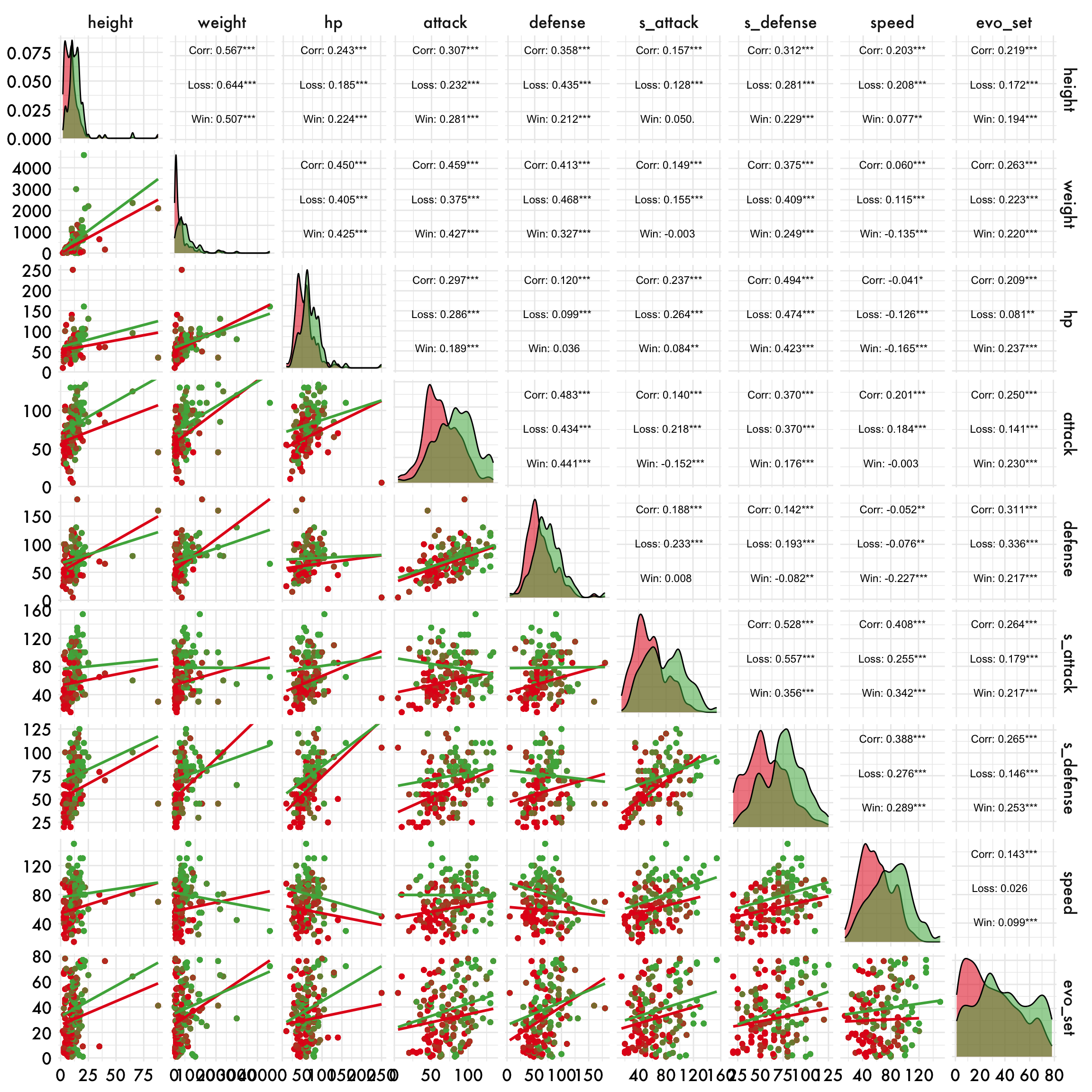

Predict Outcomes with Multilevel Binary Logistic Regression using `Specr`

Now that we have a sense of the various relationships, we can fit binary logistic regression models to predict our outcome (win/loss).

We will fit our models using a specification curve analysis (SCA) framework, via the Specr package in R. You can learn more about Specr here.

SCA will allow us to see how the model changes as we add or remove variables in a transparent manner. Briefly, SCA is a method for exploring the robustness of statistical results across different model specifications. It involves systematically varying the model’s parameters, such as the choice of predictors or the functional form, and examining how these changes affect the estimated coefficients and their significance.

The main goal is to assess whether the main findings hold up under different assumptions and to identify which specifications yield consistent results.

If you wish to learn more, you can read the following paper:

SCA-paper

Citation: Simonsohn, U., Simmons, J. P., & Nelson, L. D. (2020). Specification curve analysis. Nature Human Behaviour, 4(11), 1208–1214. https://doi.org/10.1038/s41562-020-0912-z

Write functions and prep for SCA Analysis

Before we get into the nittygritty of running analyses, we need to define some helper functions for SCA. The first one is a function to run the binomial logistic regression model. The second one is a function to extract the r-squared values from the model.

### write binomial logistic regression function to pass to specr
glmer_binomial <- possibly(
  function(formula, data) {
    require(lme4)
    require(broom.mixed)
    glmer(formula,
          data,
          family = binomial(link = "logit"),
          control = glmerControl(optimizer = "bobyqa"))
  },
  otherwise = NULL
)

tidy_new <- function(x) {
  fit <- broom::tidy(x, conf.int = TRUE)
  r2_vals <- tryCatch(
    performance::r2(x),
    error = function(e) NULL
  )
  r2_marginal <- NA
  r2_conditional <- NA
  
  if (!is.null(r2_vals)) {
    if ("R2_marginal" %in% names(r2_vals)) {
      # Mixed models: store Marginal and Conditional R2
      r2_marginal <- r2_vals$R2_marginal
      r2_conditional <- r2_vals$R2_conditional
    } else if ("R2" %in% names(r2_vals)) {
      # Simple models: store R2 in marginal, NA in conditional
      r2_marginal <- r2_vals$R2
    }
  }
  fit$res <- list(x)
  fit$r2_marginal <- r2_marginal
  fit$r2_conditional <- r2_conditional
  return(fit)
}

Set up the specifications

The Specr package allows us to set up the specifications for the models we want to run. We will set up the syntax for the models we want to run, including the variables we want to include in the model and the random effects. We will also set up a function to extract the results from the models.

The model we are trying to specify is winner ~ Predictors + (1 | challenger).

💡 In this case, we are including a random slope for the challenger variable. This means that we are allowing the effect of the challenger variable to vary across different levels of the data. This is important because it allows us to account for the fact that different challengers may have different effects on the outcome of the battle.

Here is a brief breakdown of the different arguments

data: The data frame containing the data to be analyzed.
x: The independent variables to be included in the model.
y: The dependent variable to be predicted.
model: The type of model to be used. In this case, we are using a binomial logistic regression model, which we specified earlier
controls: The control variables to be included in the model. These are the variables that we want to control for in the analysis.
add_to_formula: The random effects to be included in the model. In this case, we are including a random slope for the challenger variable.
fun1: The function to be used to extract the results from the model. In this case, we are using the broom.mixed::tidy() function to extract the results.
fun2: The function to be used to extract the r-squared values from the model. In this case, we are using the tidy_new() function we defined earlier.

### generate the different models
specs = specr::setup(
  data = df_small_scaled,
  x = c("height", "weight","attack", "defense", 
        "s_attack", "s_defense", "speed"),
  y = c('winner'),
  model = c('glmer_binomial'),
  controls = c("height", "weight","attack", "defense", 
        "s_attack", "s_defense", "speed","hp"),
add_to_formula = "(1 | challenger) ",  # Random slope
fun1 = function(x) broom.mixed::tidy(x, conf.int = TRUE),
fun2 = tidy_new
 
)

Define the formulas

Now that we have set up the specifications, we can define the formulas for the models we want to run. The specr package allows us to define the formulas for the models we want to run and extract the results in a tidy format. Use the table below to inspect the various models we aim to run.

specs$specs <- specs$specs %>%
  mutate(
    controls_sorted = sapply(strsplit(as.character(controls), ","), function(x) paste(sort(trimws(x)), collapse = ","))
  ) %>%
  distinct(x, y, model, controls_sorted, .keep_all = TRUE) %>%  # REMOVE add_to_formula
  dplyr::select(-controls_sorted)


specs$specs |> 
  dplyr::select(x, y, controls,formula) |>
  DT::datatable(
    options = list(
      pageLength = 10,
      autoWidth = TRUE,
      columnDefs = list(list(width = '200px', targets = "_all"))
    ),
    rownames = FALSE
  )

Execute the Analyses in parallel using `furrr`

Now that we have set up the specifications and defined the formulas, we can run the models.

The specr package allows us to run the models in parallel and extract the results in a tidy format, we’ll utilize furrr to run our jobs in parallel to speed up the process. We’ll also cache our output as a .RDS file, so each time we run the code, it won’t have to re-run the models.

model_path <- file.path("~/Library/CloudStorage/GoogleDrive-sm9518@princeton.edu/My Drive/Classes/Stats-blog/posts/final-project/models/sca_mode.rds") # load in the model

if (!file.exists(model_path)) { # if the file doesn't exist, then execute the code
  specs <- readRDS(model_path)
  plan() # check what plan we have
  opts <- furrr_options(
    globals = list(glmer_binomial = glmer_binomial) # tell the code we wanna use glmer 
  )
  plan(strategy = multisession, workers = 6) # switch to multisession plan to make this run faster
  results <- specr(
    specs,
    .options = opts,   # Pass opts to specr
    .progress = TRUE
  )
  plan(sequential) # switch back to sequential once done running
  saveRDS(results, model_path)
} else { # if the file exists, then load it in
  results <- readRDS(model_path)
}

View the Plots

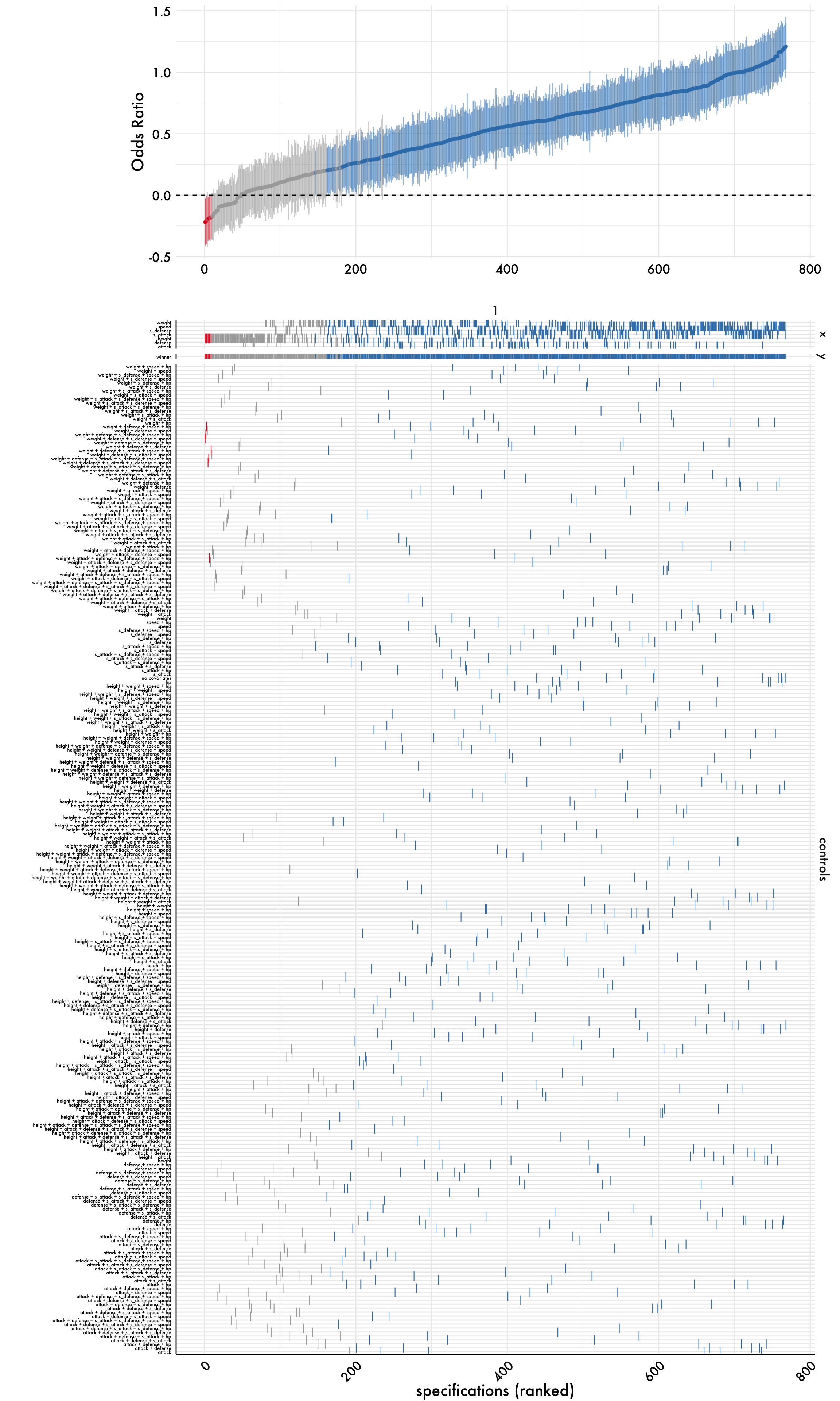
We can view our results using the plot function from specr. This simplest way to visualize most of the information contained in the results dataframe produced by our analyses. Briefly, the first plot shows the odds ratios for each model, while the second plot shows the specifications used in each model. The odds ratios are plotted on a log scale, and the confidence intervals are shown as error bars. The second plot shows the specifications used in each model, with the x-axis showing the different specifications and the y-axis showing the number of models that used that specification.

Given that we have several hundred unique models this graph gets kinda crazy to look at. You can zoom in on the plot to see the details. We’ll walk through two other ways to extract information from our results below.

p1 <- plot(results, 
           type = "curve",
           ci = T, 
           ribbon = F) +
  geom_hline(yintercept = 0, 
             linetype = "dashed", 
             color = "black") +
  labs(x = "", y = "Odds Ratio") + plot_aes

p2 <- plot(results, 
           type = "choices",
           choices = c("x", "y", "controls")) +
  labs(x = "specifications (ranked)") +
  plot_aes + 
  theme(
    axis.text.x = element_text(angle = 45, hjust = 1),
    axis.text.y = element_text(size = 5),
    axis.ticks.x = element_blank(),
    axis.ticks.y = element_blank(),
    axis.line.x = element_line("black", size = .5),
    axis.line.y = element_line("black", size = .5)
  )

plot_grid(
  p1, p2,
  ncol = 1,           
  align = "v",          
  axis = "rbl",          
  rel_heights = c(.60, 2.25)  
)

Individually Inspect the top N-Models

Now that we used specr(), we can summarize individual specifications by using broom::tidy() and broom::glance(). For most cases, this provides a sufficient and appropriate summary of the relationship of interest and model characteristics. Sometimes, however, it might be useful to investigate specific models in more detail or to investigate a specific parameter that is not provided by the two functions (e.g., r-square or variance accounted for by the model).

Inspect the significant models

First, we’ll look at just the significant models (i.e., p < 0.05). This is done by filtering the results dataframe to only include significant models. We can then use the DT package to create an interactive table that allows us to sort and filter the data.

models <- results %>% 
  as_tibble() %>% 
  dplyr::select(formula, x, y, estimate, std.error, p.value, conf.low, conf.high) %>% 
  filter(p.value < 0.051) %>%  # keep only significant models
  mutate(
    estimate = round(estimate, 3),
    std.error = round(std.error, 3),
    p.value = round(p.value, 3),
    conf.low = round(conf.low, 3),
    conf.high = round(conf.high, 3)
  ) %>%
  arrange(desc(abs(estimate)))

models |>
  DT::datatable(
    options = list(
      pageLength = 10,
      autoWidth = TRUE,
      columnDefs = list(list(targets = "_all"))
    ),
    rownames = FALSE
  )

How does R-squared change with different models?

We can also evaluate the best model by looking at the conditional r-square value. We start by ranking the models by their conditional r-square value and then plotting the results. This will allow us to see which models are the best predictors of the outcome.

From the results below, we can see that we can account for over 50% of the variance in the outcome using just the challenger Pokemon’s stats. This is a pretty good result, and it suggests that we can use these stats to predict the outcome of a battle. However, we still don’t quite know what the recipe for the best model is yet.

best_model <- results %>% 
  as_tibble() %>% 
  dplyr::select(formula, x, y, estimate, std.error, p.value, conf.low, conf.high,fit_r2_conditional) %>% 
  filter(p.value < 0.051) %>%  # keep only significant models
  mutate(
    estimate = round(estimate, 3),
    std.error = round(std.error, 3),
    p.value = round(p.value, 3),
    conf.low = round(conf.low, 3),
    conf.high = round(conf.high, 3)
  ) 

best_model %>%
  arrange(fit_r2_conditional) %>%
  mutate(rank = 1:n()) %>%
  ggplot(aes(x = rank, y = fit_r2_conditional)) +
  geom_line(color = "#ADA7C9", size = 0.85) +  # smooth teal-ish line
  geom_point(size = 1.5, alpha = 0.7, color = "#4D4861") +  # darker small points
  theme_minimal(base_family = "Futura Medium") +  # match your font
  theme(
    panel.grid.minor = element_blank(),
    panel.grid.major.x = element_blank(),
    axis.line = element_line(color = "black", size = 0.5),
    axis.ticks = element_line(color = "black"),
    axis.text = element_text(color = "black"),
    strip.text = element_blank()
  ) +
  labs(
    x = "Model Rank",
    y = "Conditional R²"
  ) +
  plot_aes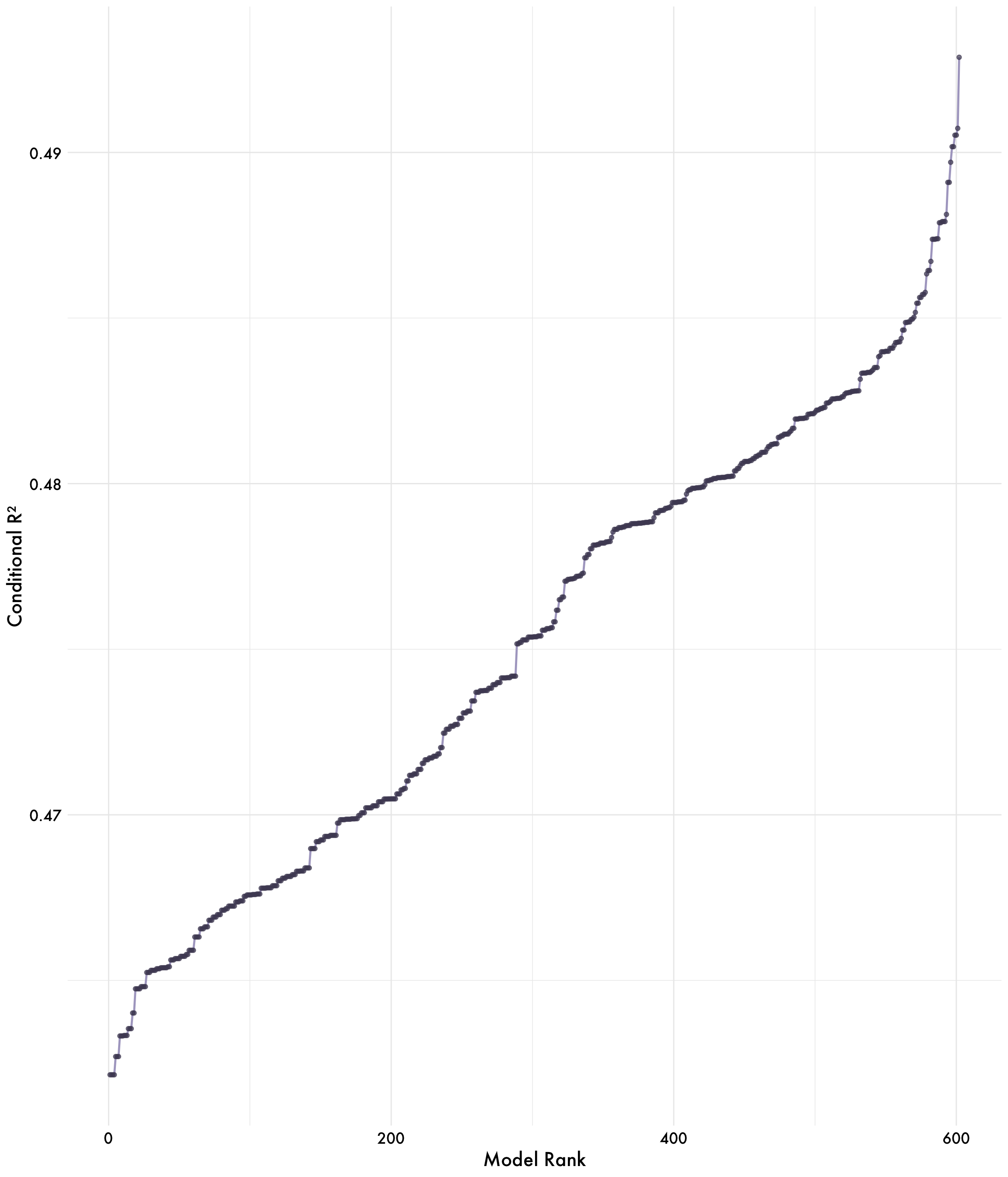

What seems to be the best model?

Now that we have a sense of the best model, we can plot the results using ggplot to create a bar graph that shows us how much variance each of the top 50 models accounts for.

best_model %>%
  arrange(desc(fit_r2_conditional), desc(estimate)) %>%
  head(50) %>%
  mutate(rank = 1:n()) %>%
  ggplot(aes(x = factor(rank), 
             y = fit_r2_conditional, 
             fill = fit_r2_conditional)) +  # Use fit_r2_conditional for color fill
  geom_col() +
  geom_text(aes(label = formula), 
            vjust = -0.5, 
            size = 3, 
            angle = 90) +
  scale_fill_gradient(low = "#ee9b00", high = "#c44536") +  # Gradient from low to high values
  plot_aes + 
  theme(
    strip.text = element_blank(),
    axis.line = element_line(color = "black", size = .5),
    axis.text = element_text(color = "black"),
    axis.text.x = element_text(angle = 45, hjust = 1),  # Rotate x-axis labels by 45 degrees
    legend.position = "none"
  ) +
  labs(x = "Model Rank", y = "Conditional R²") +
  ylim(0, 0.55)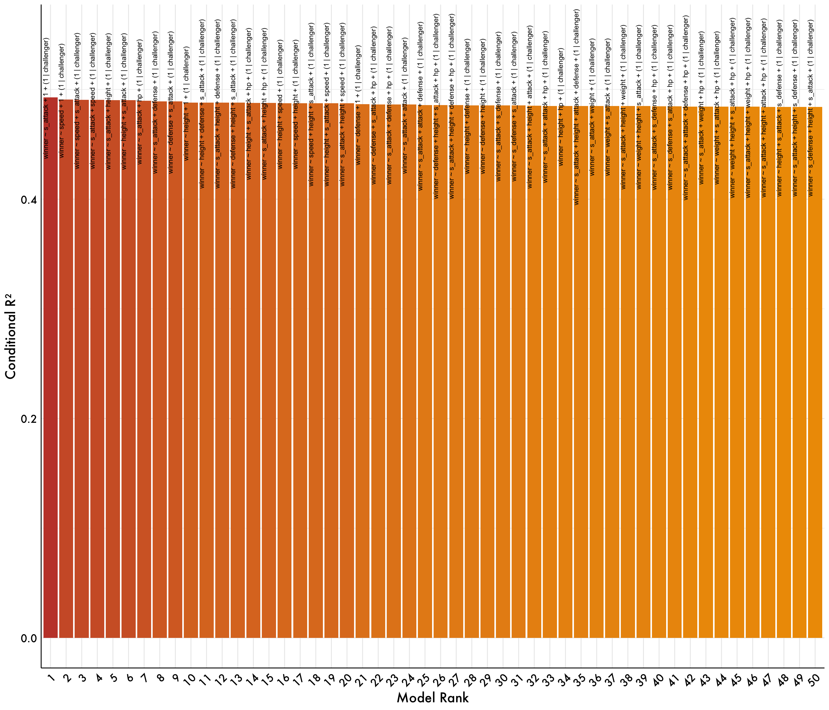

Based on what our graph tells us, the best model is (1 | challenger) + s_defense. This model accounts for 55% of the variance in the outcome, which is a pretty good result. However, it’s important to note that this is a pretty simple model and there are likely other factors that could be included to improve the model. For example, we could include the opponent’s stats or other variables that might be relevant to the outcome of the battle. If anything, this goes to show how balanced of a meta Pokemon has.

Thanks for following along!

If you’d like to learn more about SCA, I’d recommend checking out ✨Dr. Dani Cosme’s ✨ website. She’s an amazing person, teacher, and has a ton of great resources on SCA and other statistical methods in R. I especially recommend this reproducibililty workshop.

Package Citations

report::cite_packages()

  - Bates D, Mächler M, Bolker B, Walker S (2015). "Fitting Linear Mixed-Effects Models Using lme4." _Journal of Statistical Software_, *67*(1), 1-48. doi:10.18637/jss.v067.i01 <https://doi.org/10.18637/jss.v067.i01>.
  - Bates D, Maechler M, Jagan M (2024). _Matrix: Sparse and Dense Matrix Classes and Methods_. R package version 1.7-0, <https://CRAN.R-project.org/package=Matrix>.
  - Bengtsson H (2021). "A Unifying Framework for Parallel and Distributed Processing in R using Futures." _The R Journal_, *13*(2), 208-227. doi:10.32614/RJ-2021-048 <https://doi.org/10.32614/RJ-2021-048>, <https://doi.org/10.32614/RJ-2021-048>.
  - Christensen R (2023). _ordinal-Regression Models for Ordinal Data_. R package version 2023.12-4.1, <https://CRAN.R-project.org/package=ordinal>.
  - Fox J, Weisberg S (2019). _An R Companion to Applied Regression_, Third edition. Sage, Thousand Oaks CA. <https://socialsciences.mcmaster.ca/jfox/Books/Companion/>.
  - Fox J, Weisberg S, Price B (2022). _carData: Companion to Applied Regression Data Sets_. R package version 3.0-5, <https://CRAN.R-project.org/package=carData>.
  - Grolemund G, Wickham H (2011). "Dates and Times Made Easy with lubridate." _Journal of Statistical Software_, *40*(3), 1-25. <https://www.jstatsoft.org/v40/i03/>.
  - Lenth R (2025). _emmeans: Estimated Marginal Means, aka Least-Squares Means_. R package version 1.10.7, <https://CRAN.R-project.org/package=emmeans>.
  - Lüdecke D (2018). "ggeffects: Tidy Data Frames of Marginal Effects from Regression Models." _Journal of Open Source Software_, *3*(26), 772. doi:10.21105/joss.00772 <https://doi.org/10.21105/joss.00772>.
  - Lüdecke D, Ben-Shachar M, Patil I, Waggoner P, Makowski D (2021). "performance: An R Package for Assessment, Comparison and Testing of Statistical Models." _Journal of Open Source Software_, *6*(60), 3139. doi:10.21105/joss.03139 <https://doi.org/10.21105/joss.03139>.
  - Masur P, Scharkow M (2020). "specr: Conducting and Visualizing Specification Curve Analyses (Version 1.0.0)." <https://CRAN.R-project.org/package=specr>.
  - Müller K, Wickham H (2025). _tibble: Simple Data Frames_. R package version 3.3.0, <https://CRAN.R-project.org/package=tibble>.
  - R Core Team (2024). _R: A Language and Environment for Statistical Computing_. R Foundation for Statistical Computing, Vienna, Austria. <https://www.R-project.org/>.
  - Rinker TW, Kurkiewicz D (2018). _pacman: Package Management for R_. version 0.5.0, <http://github.com/trinker/pacman>.
  - Robinson D, Hayes A, Couch S (2024). _broom: Convert Statistical Objects into Tidy Tibbles_. R package version 1.0.7, <https://CRAN.R-project.org/package=broom>.
  - Schlegel B, Steenbergen M (2020). _brant: Test for Parallel Regression Assumption_. R package version 0.3-0, <https://CRAN.R-project.org/package=brant>.
  - Schloerke B, Cook D, Larmarange J, Briatte F, Marbach M, Thoen E, Elberg A, Crowley J (2024). _GGally: Extension to 'ggplot2'_. R package version 2.2.1, <https://CRAN.R-project.org/package=GGally>.
  - Vaughan D, Dancho M (2022). _furrr: Apply Mapping Functions in Parallel using Futures_. R package version 0.3.1, <https://CRAN.R-project.org/package=furrr>.
  - Venables WN, Ripley BD (2002). _Modern Applied Statistics with S_, Fourth edition. Springer, New York. ISBN 0-387-95457-0, <https://www.stats.ox.ac.uk/pub/MASS4/>.
  - Wickham H (2016). _ggplot2: Elegant Graphics for Data Analysis_. Springer-Verlag New York. ISBN 978-3-319-24277-4, <https://ggplot2.tidyverse.org>.
  - Wickham H (2023). _forcats: Tools for Working with Categorical Variables (Factors)_. R package version 1.0.0, <https://CRAN.R-project.org/package=forcats>.
  - Wickham H (2023). _stringr: Simple, Consistent Wrappers for Common String Operations_. R package version 1.5.1, <https://CRAN.R-project.org/package=stringr>.
  - Wickham H, Averick M, Bryan J, Chang W, McGowan LD, François R, Grolemund G, Hayes A, Henry L, Hester J, Kuhn M, Pedersen TL, Miller E, Bache SM, Müller K, Ooms J, Robinson D, Seidel DP, Spinu V, Takahashi K, Vaughan D, Wilke C, Woo K, Yutani H (2019). "Welcome to the tidyverse." _Journal of Open Source Software_, *4*(43), 1686. doi:10.21105/joss.01686 <https://doi.org/10.21105/joss.01686>.
  - Wickham H, François R, Henry L, Müller K, Vaughan D (2023). _dplyr: A Grammar of Data Manipulation_. R package version 1.1.4, <https://CRAN.R-project.org/package=dplyr>.
  - Wickham H, Henry L (2025). _purrr: Functional Programming Tools_. R package version 1.0.4, <https://CRAN.R-project.org/package=purrr>.
  - Wickham H, Hester J, Bryan J (2024). _readr: Read Rectangular Text Data_. R package version 2.1.5, <https://CRAN.R-project.org/package=readr>.
  - Wickham H, Vaughan D, Girlich M (2024). _tidyr: Tidy Messy Data_. R package version 1.3.1, <https://CRAN.R-project.org/package=tidyr>.
  - Xie Y, Cheng J, Tan X (2024). _DT: A Wrapper of the JavaScript Library 'DataTables'_. R package version 0.33, <https://CRAN.R-project.org/package=DT>.

Overview

Load packages:

GPT Pipeline

Load Libraries, API Key, and set model information

Load Data and Sample

Hit the API to Simulate Match-ups

Load Curated Dataset

Take a look at the data

Exploratory Data Analysis

Visualize the distribution of the various Pokémon stats

Distribution of Pokémon stats

Comparing Distributions of Pokémon stats by outcome

Comparing Relations between variables and outcomes

Predict Outcomes with Multilevel Binary Logistic Regression using Specr

Write functions and prep for SCA Analysis

Set up the specifications

Define the formulas

Execute the Analyses in parallel using furrr

View the Plots

Individually Inspect the top N-Models

Inspect the significant models

How does R-squared change with different models?

What seems to be the best model?

Package Citations

Predict Outcomes with Multilevel Binary Logistic Regression using `Specr`

Execute the Analyses in parallel using `furrr`